8 Sampling

Sampling is the statistical process of selecting a subset—called a ‘sample’—of a population of interest for the purpose of making observations and statistical inferences about that population. Social science research is generally about inferring patterns of behaviours within specific populations. We cannot study entire populations because of feasibility and cost constraints, and hence, we must select a representative sample from the population of interest for observation and analysis. It is extremely important to choose a sample that is truly representative of the population so that the inferences derived from the sample can be generalised back to the population of interest. Improper and biased sampling is the primary reason for the often divergent and erroneous inferences reported in opinion polls and exit polls conducted by different polling groups such as CNN/Gallup Poll, ABC, and CBS, prior to every US Presidential election.

The sampling process

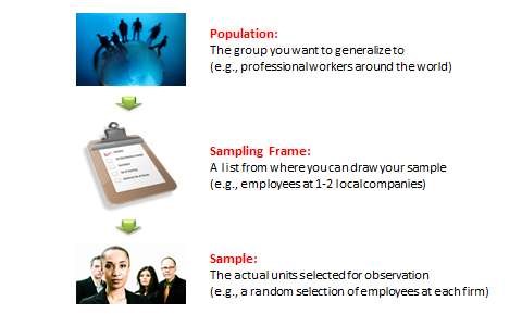
As Figure 8.1 shows, the sampling process comprises of several stages. The first stage is defining the target population. A population can be defined as all people or items (unit of analysis) with the characteristics that one wishes to study. The unit of analysis may be a person, group, organisation, country, object, or any other entity that you wish to draw scientific inferences about. Sometimes the population is obvious. For example, if a manufacturer wants to determine whether finished goods manufactured at a production line meet certain quality requirements or must be scrapped and reworked, then the population consists of the entire set of finished goods manufactured at that production facility. At other times, the target population may be a little harder to understand. If you wish to identify the primary drivers of academic learning among high school students, then what is your target population: high school students, their teachers, school principals, or parents? The right answer in this case is high school students, because you are interested in their performance, not the performance of their teachers, parents, or schools. Likewise, if you wish to analyse the behaviour of roulette wheels to identify biased wheels, your population of interest is not different observations from a single roulette wheel, but different roulette wheels (i.e., their behaviour over an infinite set of wheels).

The second step in the sampling process is to choose a sampling frame. This is an accessible section of the target population—usually a list with contact information—from where a sample can be drawn. If your target population is professional employees at work, because you cannot access all professional employees around the world, a more realistic sampling frame will be employee lists of one or two local companies that are willing to participate in your study. If your target population is organisations, then the Fortune 500 list of firms or the Standard & Poor’s (S&P) list of firms registered with the New York Stock exchange may be acceptable sampling frames.

Note that sampling frames may not entirely be representative of the population at large, and if so, inferences derived by such a sample may not be generalisable to the population. For instance, if your target population is organisational employees at large (e.g., you wish to study employee self-esteem in this population) and your sampling frame is employees at automotive companies in the American Midwest, findings from such groups may not even be generalisable to the American workforce at large, let alone the global workplace. This is because the American auto industry has been under severe competitive pressures for the last 50 years and has seen numerous episodes of reorganisation and downsizing, possibly resulting in low employee morale and self-esteem. Furthermore, the majority of the American workforce is employed in service industries or in small businesses, and not in automotive industry. Hence, a sample of American auto industry employees is not particularly representative of the American workforce. Likewise, the Fortune 500 list includes the 500 largest American enterprises, which is not representative of all American firms, most of which are medium or small sized firms rather than large firms, and is therefore, a biased sampling frame. In contrast, the S&P list will allow you to select large, medium, and/or small companies, depending on whether you use the S&P LargeCap, MidCap, or SmallCap lists, but includes publicly traded firms (and not private firms) and is hence still biased. Also note that the population from which a sample is drawn may not necessarily be the same as the population about which we actually want information. For example, if a researcher wants to examine the success rate of a new ‘quit smoking’ program, then the target population is the universe of smokers who had access to this program, which may be an unknown population. Hence, the researcher may sample patients arriving at a local medical facility for smoking cessation treatment, some of whom may not have had exposure to this particular ‘quit smoking’ program, in which case, the sampling frame does not correspond to the population of interest.

The last step in sampling is choosing a sample from the sampling frame using a well-defined sampling technique. Sampling techniques can be grouped into two broad categories: probability (random) sampling and non-probability sampling. Probability sampling is ideal if generalisability of results is important for your study, but there may be unique circumstances where non-probability sampling can also be justified. These techniques are discussed in the next two sections.

Probability sampling

Probability sampling is a technique in which every unit in the population has a chance (non-zero probability) of being selected in the sample, and this chance can be accurately determined. Sample statistics thus produced, such as sample mean or standard deviation, are unbiased estimates of population parameters, as long as the sampled units are weighted according to their probability of selection. All probability sampling have two attributes in common: every unit in the population has a known non-zero probability of being sampled, and the sampling procedure involves random selection at some point. The different types of probability sampling techniques include:

Simple random sampling. In this technique, all possible subsets of a population (more accurately, of a sampling frame) are given an equal probability of being selected The probability of selecting any set of \(n\) units out of a total of \(N\) units in a sampling frame is \({}^{N}C_{n} \). Hence, sample statistics are unbiased estimates of population parameters, without any weighting. Simple random sampling involves randomly selecting respondents from a sampling frame, but with large sampling frames, usually a table of random numbers or a computerised random number generator is used. For instance, if you wish to select 200 firms to survey from a list of 1,000 firms, if this list is entered into a spreadsheet like Excel, you can use Excel’s RAND() function to generate random numbers for each of the 1,000 clients on that list. Next, you sort the list in increasing order of their corresponding random number, and select the first 200 clients on that sorted list. This is the simplest of all probability sampling techniques, however, the simplicity is also the strength of this technique. Because the sampling frame is not subdivided or partitioned, the sample is unbiased and the inferences are most generalisable amongst all probability sampling techniques.

Systematic sampling. In this technique, the sampling frame is ordered according to some criteria and elements selected at regular intervals through that ordered list. Systematic sampling involves a random start and then proceeds with the selection of every \(k\)^th element from that point onwards, where \(k = N/n\), where \(k\) is the ratio of sampling frame size \(N\) and the desired sample size \(n\), and is formally called the sampling ratio. It is important that the starting point is not automatically the first in the list, but is instead randomly chosen from within the first \(k\) elements on the list. In our previous example of selecting 200 firms from a list of 1,000 firms, you can sort the 1,000 firms in increasing (or decreasing) order of their size (i.e., employee count or annual revenues), randomly select one of the first five firms on the sorted list, and then select every fifth firm on the list. This process will ensure that there is no over-representation of large or small firms in your sample, but rather that firms of all sizes are generally uniformly represented, as it is in your sampling frame. In other words, the sample is representative of the population, at least on the basis of the sorting criterion.

Stratified sampling. In stratified sampling, the sampling frame is divided into homogeneous and non-overlapping subgroups (called ‘strata’), and a simple random sample is drawn within each subgroup. In the previous example of selecting 200 firms from a list of 1,000 firms, you can start by categorising the firms based on their size as large (more than 500 employees), medium (between 50 and 500 employees), and small (less than 50 employees). You can then randomly select 67 firms from each subgroup to make up your sample of 200 firms. However, since there are many more small firms in a sampling frame than large firms, having an equal number of small, medium, and large firms will make the sample less representative of the population (i.e., biased in favour of large firms that are fewer in number in the target population). This is called non-proportional stratified sampling because the proportion of the sample within each subgroup does not reflect the proportions in the sampling frame—or the population of interest—and the smaller subgroup (large-sized firms) is oversampled. An alternative technique will be to select subgroup samples in proportion to their size in the population. For instance, if there are 100 large firms, 300 mid-sized firms, and 600 small firms, you can sample 20 firms from the ‘large’ group, 60 from the ‘medium’ group and 120 from the ‘small’ group. In this case, the proportional distribution of firms in the population is retained in the sample, and hence this technique is called proportional stratified sampling. Note that the non-proportional approach is particularly effective in representing small subgroups, such as large-sized firms, and is not necessarily less representative of the population compared to the proportional approach, as long as the findings of the non-proportional approach are weighted in accordance to a subgroup’s proportion in the overall population.

Cluster sampling. If you have a population dispersed over a wide geographic region, it may not be feasible to conduct a simple random sampling of the entire population. In such case, it may be reasonable to divide the population into ‘clusters’—usually along geographic boundaries—randomly sample a few clusters, and measure all units within that cluster. For instance, if you wish to sample city governments in the state of New York, rather than travel all over the state to interview key city officials (as you may have to do with a simple random sample), you can cluster these governments based on their counties, randomly select a set of three counties, and then interview officials from every office in those counties. However, depending on between-cluster differences, the variability of sample estimates in a cluster sample will generally be higher than that of a simple random sample, and hence the results are less generalisable to the population than those obtained from simple random samples.

Matched-pairs sampling. Sometimes, researchers may want to compare two subgroups within one population based on a specific criterion. For instance, why are some firms consistently more profitable than other firms? To conduct such a study, you would have to categorise a sampling frame of firms into ‘high profitable’ firms and ‘low profitable firms’ based on gross margins, earnings per share, or some other measure of profitability. You would then select a simple random sample of firms in one subgroup, and match each firm in this group with a firm in the second subgroup, based on its size, industry segment, and/or other matching criteria. Now, you have two matched samples of high-profitability and low-profitability firms that you can study in greater detail. Matched-pairs sampling techniques are often an ideal way of understanding bipolar differences between different subgroups within a given population.

Multi-stage sampling. The probability sampling techniques described previously are all examples of single-stage sampling techniques. Depending on your sampling needs, you may combine these single-stage techniques to conduct multi-stage sampling. For instance, you can stratify a list of businesses based on firm size, and then conduct systematic sampling within each stratum. This is a two-stage combination of stratified and systematic sampling. Likewise, you can start with a cluster of school districts in the state of New York, and within each cluster, select a simple random sample of schools. Within each school, you can select a simple random sample of grade levels, and within each grade level, you can select a simple random sample of students for study. In this case, you have a four-stage sampling process consisting of cluster and simple random sampling.

Non-probability sampling

Non-probability sampling is a sampling technique in which some units of the population have zero chance of selection or where the probability of selection cannot be accurately determined. Typically, units are selected based on certain non-random criteria, such as quota or convenience. Because selection is non-random, non-probability sampling does not allow the estimation of sampling errors, and may be subjected to a sampling bias. Therefore, information from a sample cannot be generalised back to the population. Types of non-probability sampling techniques include:

Convenience sampling. Also called accidental or opportunity sampling, this is a technique in which a sample is drawn from that part of the population that is close to hand, readily available, or convenient. For instance, if you stand outside a shopping centre and hand out questionnaire surveys to people or interview them as they walk in, the sample of respondents you will obtain will be a convenience sample. This is a non-probability sample because you are systematically excluding all people who shop at other shopping centres. The opinions that you would get from your chosen sample may reflect the unique characteristics of this shopping centre such as the nature of its stores (e.g., high end-stores will attract a more affluent demographic), the demographic profile of its patrons, or its location (e.g., a shopping centre close to a university will attract primarily university students with unique purchasing habits), and therefore may not be representative of the opinions of the shopper population at large. Hence, the scientific generalisability of such observations will be very limited. Other examples of convenience sampling are sampling students registered in a certain class or sampling patients arriving at a certain medical clinic. This type of sampling is most useful for pilot testing, where the goal is instrument testing or measurement validation rather than obtaining generalisable inferences.

Quota sampling. In this technique, the population is segmented into mutually exclusive subgroups (just as in stratified sampling), and then a non-random set of observations is chosen from each subgroup to meet a predefined quota. In proportional quota sampling, the proportion of respondents in each subgroup should match that of the population. For instance, if the American population consists of 70 per cent Caucasians, 15 per cent Hispanic-Americans, and 13 per cent African-Americans, and you wish to understand their voting preferences in an sample of 98 people, you can stand outside a shopping centre and ask people their voting preferences. But you will have to stop asking Hispanic-looking people when you have 15 responses from that subgroup (or African-Americans when you have 13 responses) even as you continue sampling other ethnic groups, so that the ethnic composition of your sample matches that of the general American population.

Non-proportional quota sampling is less restrictive in that you do not have to achieve a proportional representation, but perhaps meet a minimum size in each subgroup. In this case, you may decide to have 50 respondents from each of the three ethnic subgroups (Caucasians, Hispanic-Americans, and African-Americans), and stop when your quota for each subgroup is reached. Neither type of quota sampling will be representative of the American population, since depending on whether your study was conducted in a shopping centre in New York or Kansas, your results may be entirely different. The non-proportional technique is even less representative of the population, but may be useful in that it allows capturing the opinions of small and under-represented groups through oversampling.

Expert sampling. This is a technique where respondents are chosen in a non-random manner based on their expertise on the phenomenon being studied. For instance, in order to understand the impacts of a new governmental policy such as the Sarbanes-Oxley Act, you can sample a group of corporate accountants who are familiar with this Act. The advantage of this approach is that since experts tend to be more familiar with the subject matter than non-experts, opinions from a sample of experts are more credible than a sample that includes both experts and non-experts, although the findings are still not generalisable to the overall population at large.

Snowball sampling. In snowball sampling, you start by identifying a few respondents that match the criteria for inclusion in your study, and then ask them to recommend others they know who also meet your selection criteria. For instance, if you wish to survey computer network administrators and you know of only one or two such people, you can start with them and ask them to recommend others who also work in network administration. Although this method hardly leads to representative samples, it may sometimes be the only way to reach hard-to-reach populations or when no sampling frame is available.

Statistics of sampling

In the preceding sections, we introduced terms such as population parameter, sample statistic, and sampling bias. In this section, we will try to understand what these terms mean and how they are related to each other.

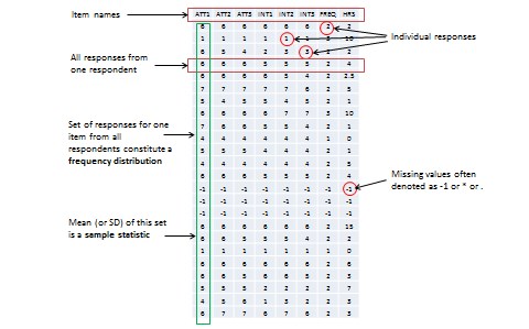
When you measure a certain observation from a given unit, such as a person’s response to a Likert-scaled item, that observation is called a response (see Figure 8.2). In other words, a response is a measurement value provided by a sampled unit. Each respondent will give you different responses to different items in an instrument. Responses from different respondents to the same item or observation can be graphed into a frequency distribution based on their frequency of occurrences. For a large number of responses in a sample, this frequency distribution tends to resemble a bell-shaped curve called a normal distribution, which can be used to estimate overall characteristics of the entire sample, such as sample mean (average of all observations in a sample) or standard deviation (variability or spread of observations in a sample). These sample estimates are called sample statistics (a ‘statistic’ is a value that is estimated from observed data). Populations also have means and standard deviations that could be obtained if we could sample the entire population. However, since the entire population can never be sampled, population characteristics are always unknown, and are called population parameters (and not ‘statistic’ because they are not statistically estimated from data). Sample statistics may differ from population parameters if the sample is not perfectly representative of the population. The difference between the two is called sampling error. Theoretically, if we could gradually increase the sample size so that the sample approaches closer and closer to the population, then sampling error will decrease and a sample statistic will increasingly approximate the corresponding population parameter.

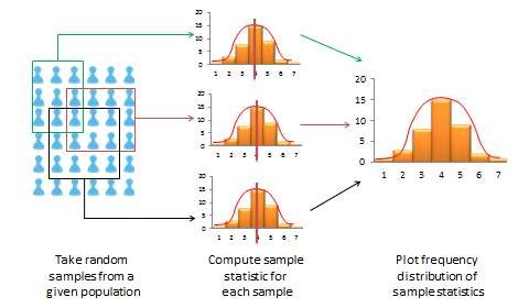
If a sample is truly representative of the population, then the estimated sample statistics should be identical to the corresponding theoretical population parameters. How do we know if the sample statistics are at least reasonably close to the population parameters? Here, we need to understand the concept of a sampling distribution. Imagine that you took three different random samples from a given population, as shown in Figure 8.3, and for each sample, you derived sample statistics such as sample mean and standard deviation. If each random sample was truly representative of the population, then your three sample means from the three random samples will be identical—and equal to the population parameter—and the variability in sample means will be zero. But this is extremely unlikely, given that each random sample will likely constitute a different subset of the population, and hence, their means may be slightly different from each other. However, you can take these three sample means and plot a frequency histogram of sample means. If the number of such samples increases from three to 10 to 100, the frequency histogram becomes a sampling distribution. Hence, a sampling distribution is a frequency distribution of a sample statistic (like sample mean) from a set of samples, while the commonly referenced frequency distribution is the distribution of a response (observation) from a single sample. Just like a frequency distribution, the sampling distribution will also tend to have more sample statistics clustered around the mean (which presumably is an estimate of a population parameter), with fewer values scattered around the mean. With an infinitely large number of samples, this distribution will approach a normal distribution. The variability or spread of a sample statistic in a sampling distribution (i.e., the standard deviation of a sampling statistic) is called its standard error. In contrast, the term standard deviation is reserved for variability of an observed response from a single sample.

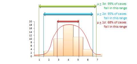
The mean value of a sample statistic in a sampling distribution is presumed to be an estimate of the unknown population parameter. Based on the spread of this sampling distribution (i.e., based on standard error), it is also possible to estimate confidence intervals for that prediction population parameter. Confidence interval is the estimated probability that a population parameter lies within a specific interval of sample statistic values. All normal distributions tend to follow a 68–95–99%  rule (see Figure 8.4), which says that over 68% of the cases in the distribution lie within one standard deviation of the mean value \((\mu + 1\sigma)\), over 95% of the cases in the distribution lie within two standard deviations of the mean \((\mu + 2\sigma)\), and over 99% of the cases in the distribution lie within three standard deviations of the mean value \((\mu + 3\sigma)\). Since a sampling distribution with an infinite number of samples will approach a normal distribution, the same 68-95-99% rule applies, and it can be said that:

(Sample statistic \(\pm\) one standard error) represents a 68% confidence interval for the population parameter.

(Sample statistic \(\pm\) two standard errors) represents a 95% confidence interval for the population parameter.

(Sample statistic \(\pm\) three standard errors) represents a 99% confidence interval for the population parameter.

A sample is ‘biased’ (i.e., not representative of the population) if its sampling distribution cannot be estimated or if the sampling distribution violates the 68–95–99%  rule. As an aside, note that in most regression analysis where we examine the significance of regression coefficients with \(p<0.05\), we are attempting to see if the sampling statistic (regression coefficient) predicts the corresponding population parameter (true effect size) with a 95% confidence interval. Interestingly, the ‘six sigma’ standard attempts to identify manufacturing defects outside the 99% confidence interval or six standard deviations (standard deviation is represented using the Greek letter sigma), representing significance testing at \(p<0.01\).