7 Scale reliability and validity

The previous chapter examined some of the difficulties with measuring constructs in social science research. For instance, how do we know whether we are measuring ‘compassion’ and not ‘empathy’, since both constructs are somewhat similar in meaning? Or is compassion the same thing as empathy? What makes it more complex is that sometimes these constructs are imaginary concepts (i.e., they do not exist in reality), and multidimensional (in which case, we have the added problem of identifying their constituent dimensions). Hence, it is not adequate just to measure social science constructs using any scale that we prefer. We also must test these scales to ensure that: they indeed measure the unobservable construct that we wanted to measure (i.e., the scales are ‘valid’), and they measure the intended construct consistently and precisely (i.e., the scales are ‘reliable’). Reliability and validity—jointly called the ‘psychometric properties’ of measurement scales—are the yardsticks against which the adequacy and accuracy of our measurement procedures are evaluated in scientific research.

A measure can be reliable but not valid if it is measuring something very consistently, but is consistently measuring the wrong construct. Likewise, a measure can be valid but not reliable if it is measuring the right construct, but not doing so in a consistent manner. Using the analogy of a shooting target, as shown in Figure 7.1, a multiple-item measure of a construct that is both reliable and valid consists of shots that cluster within a narrow range near the centre of the target. A measure that is valid but not reliable will consist of shots centred on the target but not clustered within a narrow range, but rather scattered around the target. Finally, a measure that is reliable but not valid will consist of shots clustered within a narrow range but away from the centre of the target. Hence, reliability and validity are both needed to ensure adequate measurement of the constructs of interest.

Reliability

Reliability is the degree to which the measure of a construct is consistent or dependable. In other words, if we use this scale to measure the same construct multiple times, do we get pretty much the same result every time, assuming the underlying phenomenon is not changing? An example of an unreliable measurement is people guessing your weight. Quite likely, people will guess differently, the different measures will be inconsistent, and therefore, the ‘guessing’ technique of measurement is unreliable. A more reliable measurement may be to use a weight scale, where you are likely to get the same value every time you step on the scale, unless your weight has actually changed between measurements.

Note that reliability implies consistency but not accuracy. In the previous example of the weight scale, if the weight scale is calibrated incorrectly—say, to shave ten pounds off your true weight, just to make you feel better—it will not measure your true weight and is therefore not a valid measure. Nevertheless, the miscalibrated weight scale will still give you the same weight every time (which is ten pounds less than your true weight), and hence the scale is reliable.

What are the sources of unreliable observations in social science measurements? One of the primary sources is the observer’s—or researcher’s—subjectivity. If employee morale in a firm is measured by watching whether the employees smile at each other, whether they make jokes, and so forth, then different observers may infer different measures of morale if they are watching the employees on a very busy day (when they have no time to joke or chat) or a light day (when they are more jovial or chatty). Two observers may also infer different levels of morale on the same day, depending on what they view as a joke and what is not. ‘Observation’ is a qualitative measurement technique. Sometimes, reliability may be improved by using quantitative measures—for instance, by counting the number of grievances filed over one month as a measure of the inverse of morale. Of course, grievances may or may not be a valid measure of morale, but it is less subject to human subjectivity, and therefore more reliable. A second source of unreliable observation is asking imprecise or ambiguous questions. For instance, if you ask people what their salary is, different respondents may interpret this question differently as monthly salary, annual salary, or per hour wage, and hence, the resulting observations will likely be highly divergent and unreliable. A third source of unreliability is asking questions about issues that respondents are not very familiar with or do not care about, such as asking an American college graduate whether they are satisfied with Canada’s relationship with Slovenia, or asking a Chief Executive Officer to rate the effectiveness of their company’s technology strategy—something that they have likely delegated to a technology executive.

So how can you create reliable measures? If your measurement involves soliciting information from others—as is the case with much of social science research—then you can start by replacing data collection techniques that depend more on researcher subjectivity (such as observations) with those that are less dependent on subjectivity (such as questionnaires), by asking only those questions that respondents may know the answer to or issues that they care about, by avoiding ambiguous items in your measures (e.g., by clearly stating whether you are looking for annual salary), and by simplifying the wording in your indicators so that they are not misinterpreted by some respondents (e.g., by avoiding difficult words whose meanings they may not know). These strategies can improve the reliability of our measures, even though they will not necessarily make the measurements completely reliable. Measurement instruments must still be tested for reliability. There are many ways of estimating reliability, which are discussed next.

Inter-rater reliability. Inter-rater reliability—also called inter-observer reliability—is a measure of consistency between two or more independent raters (observers) of the same construct. Usually, this is assessed in a pilot study, and can be done in two ways, depending on the level of measurement of the construct. If the measure is categorical, a set of all categories is defined, raters check off which category each observation falls in, and the percentage of agreement between the raters is an estimate of inter-rater reliability. For instance, if there are two raters rating 100 observations into one of three possible categories, and their ratings match for 75 per cent of the observations, then inter-rater reliability is 0.75. If the measure is interval or ratio scaled (e.g., classroom activity is being measured once every five minutes by two raters on a 1 to 7 response scale), then a simple correlation between measures from the two raters can also serve as an estimate of inter-rater reliability.

Test-retest reliability. Test-retest reliability is a measure of consistency between two measurements (tests) of the same construct administered to the same sample at two different points in time. If the observations have not changed substantially between the two tests, then the measure is reliable. The correlation in observations between the two tests is an estimate of test-retest reliability. Note here that the time interval between the two tests is critical. Generally, the longer the time gap, the greater the chance that the two observations may change during this time (due to random error), and the lower the test-retest reliability will be.

Split-half reliability. Split-half reliability is a measure of consistency between two halves of a construct measure. For instance, if you have a ten-item measure of a given construct, randomly split those ten items into two sets of five (unequal halves are allowed if the total number of items is odd), and administer the entire instrument to a sample of respondents. Then, calculate the total score for each half for each respondent, and the correlation between the total scores in each half is a measure of split-half reliability. The longer the instrument, the more likely it is that the two halves of the measure will be similar (since random errors are minimised as more items are added), and hence, this technique tends to systematically overestimate the reliability of longer instruments.

Internal consistency reliability. Internal consistency reliability is a measure of consistency between different items of the same construct. If a multiple-item construct measure is administered to respondents, the extent to which respondents rate those items in a similar manner is a reflection of internal consistency. This reliability can be estimated in terms of average inter-item correlation, average item-to-total correlation, or more commonly, Cronbach’s alpha. As an example, if you have a scale with six items, you will have fifteen different item pairings, and fifteen correlations between these six items. Average inter-item correlation is the average of these fifteen correlations. To calculate average item-to-total correlation, you have to first create a ‘total’ item by adding the values of all six items, compute the correlations between this total item and each of the six individual items, and finally, average the six correlations. Neither of the two above measures takes into account the number of items in the measure (six items in this example). Cronbach’s alpha, a reliability measure designed by Lee Cronbach in 1951, factors in scale size in reliability estimation, calculated using the following formula:

\[ \alpha=\frac{K}{K-1}\left(1-\frac{\sum^{K}_{i=1}\sigma^{2}_{Y_i}}{\sigma^{2}_{X}} \right) \]

where \(K\) is the number of items in the measure, \(\sigma^{2}_{X}\) is the variance (square of standard deviation) of the observed total scores, and \(\sigma^{2}_{Y_i}\) is the observed variance for item \(i\). The standardised Cronbach’s alpha can be computed using a simpler formula:

\[\alpha_{\mbox{standardised}}=\frac{K_{\bar{r}}}{(1+(K-1)\bar{r})} \]

where \(K\) is the number of items, \(\bar{r}\) is the average inter-item correlation—i.e., the mean of \(K(K-1)/2\) coefficients in the upper triangular (or lower triangular) correlation matrix.

Validity

Validity, often called construct validity, refers to the extent to which a measure adequately represents the underlying construct that it is supposed to measure. For instance, is a measure of compassion really measuring compassion, and not measuring a different construct such as empathy? Validity can be assessed using theoretical or empirical approaches, and should ideally be measured using both approaches. Theoretical assessment of validity focuses on how well the idea of a theoretical construct is translated into or represented in an operational measure. This type of validity is called translational validity (or representational validity), and consists of two subtypes: face and content validity. Translational validity is typically assessed using a panel of expert judges, who rate each item (indicator) on how well they fit the conceptual definition of that construct, and a qualitative technique called Q-sort.

Empirical assessment of validity examines how well a given measure relates to one or more external criterion, based on empirical observations. This type of validity is called criterion-related validity, which includes four subtypes: convergent, discriminant, concurrent, and predictive validity. While translation validity examines whether a measure is a good reflection of its underlying construct, criterion-related validity examines whether a given measure behaves the way it should, given the theory of that construct. This assessment is based on quantitative analysis of observed data using statistical techniques such as correlational analysis, factor analysis, and so forth. The distinction between theoretical and empirical assessment of validity is illustrated in Figure 7.2. However, both approaches are needed to adequately ensure the validity of measures in social science research.

Note that the different types of validity discussed here refer to the validity of the measurement procedures, which is distinct from the validity of hypotheses testing procedures, such as internal validity (causality), external validity (generalisability), or statistical conclusion validity. The latter types of validity are discussed in a later chapter.

Face validity. Face validity refers to whether an indicator seems to be a reasonable measure of its underlying construct ‘on its face’. For instance, the frequency of one’s attendance at religious services seems to make sense as an indication of a person’s religiosity without a lot of explanation. Hence this indicator has face validity. However, if we were to suggest how many books were checked out of an office library as a measure of employee morale, then such a measure would probably lack face validity because it does not seem to make much sense. Interestingly, some of the popular measures used in organisational research appear to lack face validity. For instance, absorptive capacity of an organisation (how much new knowledge it can assimilate for improving organisational processes) has often been measured as research and development intensity (i.e., R&D expenses divided by gross revenues)! If your research includes constructs that are highly abstract or constructs that are hard to conceptually separate from each other (e.g., compassion and empathy), it may be worthwhile to consider using a panel of experts to evaluate the face validity of your construct measures.

Content validity. Content validity is an assessment of how well a set of scale items matches with the relevant content domain of the construct that it is trying to measure. For instance, if you want to measure the construct ‘satisfaction with restaurant service’, and you define the content domain of restaurant service as including the quality of food, courtesy of wait staff, duration of wait, and the overall ambience of the restaurant (i.e., whether it is noisy, smoky, etc.), then for adequate content validity, this construct should be measured using indicators that examine the extent to which a restaurant patron is satisfied with the quality of food, courtesy of wait staff, length of wait, and the restaurant’s ambience. Of course, this approach requires a detailed description of the entire content domain of a construct, which may be difficult for complex constructs such as self-esteem or intelligence. Hence, it may not be always possible to adequately assess content validity. As with face validity, an expert panel of judges may be employed to examine content validity of constructs.

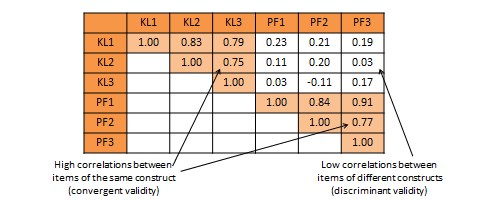
Convergent validity refers to the closeness with which a measure relates to (or converges on) the construct that it is purported to measure, and discriminant validity refers to the degree to which a measure does not measure (or discriminates from) other constructs that it is not supposed to measure. Usually, convergent validity and discriminant validity are assessed jointly for a set of related constructs. For instance, if you expect that an organisation’s knowledge is related to its performance, how can you ensure that your measure of organisational knowledge is indeed measuring organisational knowledge (for convergent validity) and not organisational performance (for discriminant validity)? Convergent validity can be established by comparing the observed values of one indicator of one construct with that of other indicators of the same construct and demonstrating similarity (or high correlation) between values of these indicators. Discriminant validity is established by demonstrating that indicators of one construct are dissimilar from (i.e., have low correlation with) other constructs. In the above example, if we have a three-item measure of organisational knowledge and three more items for organisational performance, based on observed sample data, we can compute bivariate correlations between each pair of knowledge and performance items. If this correlation matrix shows high correlations within items of the organisational knowledge and organisational performance constructs, but low correlations between items of these constructs, then we have simultaneously demonstrated convergent and discriminant validity (see Table 7.1).

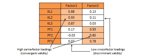
An alternative and more common statistical method used to demonstrate convergent and discriminant validity is exploratory factor analysis. This is a data reduction technique which aggregates a given set of items to a smaller set of factors based on the bivariate correlation structure discussed above using a statistical technique called principal components analysis. These factors should ideally correspond to the underlying theoretical constructs that we are trying to measure. The general norm for factor extraction is that each extracted factor should have an eigenvalue greater than 1.0. The extracted factors can then be rotated using orthogonal or oblique rotation techniques, depending on whether the underlying constructs are expected to be relatively uncorrelated or correlated, to generate factor weights that can be used to aggregate the individual items of each construct into a composite measure. For adequate convergent validity, it is expected that items belonging to a common construct should exhibit factor loadings of 0.60 or higher on a single factor (called same-factor loadings), while for discriminant validity, these items should have factor loadings of 0.30 or less on all other factors (cross-factor loadings), as shown in the rotated factor matrix example in Table 7.2. A more sophisticated technique for evaluating convergent and discriminant validity is the multi-trait multi-method (MTMM) approach. This technique requires measuring each construct (trait) using two or more different methods (e.g., survey and personal observation, or perhaps survey of two different respondent groups such as teachers and parents for evaluating academic quality). This is an onerous and relatively less popular approach, and is therefore not discussed here.

Criterion-related validity can also be assessed based on whether a given measure relates well with a current or future criterion, which are respectively called concurrent and predictive validity. Predictive validity is the degree to which a measure successfully predicts a future outcome that it is theoretically expected to predict. For instance, can standardised test scores (e.g., Scholastic Aptitude Test scores) correctly predict academic success in university (e.g., as measured by GPA)? Assessing such validity requires creation of a ‘nomological network’ showing how constructs are theoretically related to each other. Concurrent validity examines how well one measure relates to other concrete criterion that is presumed to occur simultaneously. For instance, do students’ scores in a calculus class correlate well with their scores in a linear algebra class? These scores should be related concurrently because they are both tests of mathematics. Unlike convergent and discriminant validity, concurrent and predictive validity is frequently ignored in empirical social science research.

Theory of measurement

Now that we know the different kinds of reliability and validity, let us try to synthesise our understanding of reliability and validity in a mathematical manner using classical test theory, also called true score theory. This is a psychometric theory that examines how measurement works, what it measures, and what it does not measure. This theory postulates that every observation has a true score \(T\) that can be observed accurately if there were no errors in measurement. However, the presence of measurement errors \(E\) results in a deviation of the observed score \(X\) from the true score as follows:

Observed score = True score + Error

\[X = T  + E\,.\]

Across a set of observed scores, the variance of observed and true scores can be related using a similar equation:

\[\mbox{var}(X) = \mbox{var}(T) + \mbox{var}(E)\,. \]

The goal of psychometric analysis is to estimate and minimise if possible the error variance \(\mbox{var}(E)\), so that the observed score \(X\) is a good measure of the true score \(T\).

Measurement errors can be of two types: random error and systematic error. Random error is the error that can be attributed to a set of unknown and uncontrollable external factors that randomly influence some observations but not others. As an example, during the time of measurement, some respondents may be in a nicer mood than others, which may influence how they respond to the measurement items. For instance, respondents in a nicer mood may respond more positively to constructs like self-esteem, satisfaction, and happiness than those who are in a poor mood. However, it is not possible to anticipate which subject is in what type of mood or control for the effect of mood in research studies. Likewise, at an organisational level, if we are measuring firm performance, regulatory or environmental changes may affect the performance of some firms in an observed sample but not others. Hence, random error is considered to be ‘noise’ in measurement and generally ignored.

Systematic error is an error that is introduced by factors that systematically affect all observations of a construct across an entire sample in a systematic manner. In our previous example of firm performance, since the recent financial crisis impacted the performance of financial firms disproportionately more than any other type of firms such as manufacturing or service firms, if our sample consisted only of financial firms, we may expect a systematic reduction in performance of all firms in our sample due to the financial crisis. Unlike random error, which may be positive negative, or zero, across observation in a sample, systematic errors tends to be consistently positive or negative across the entire sample. Hence, systematic error is sometimes considered to be ‘bias’ in measurement and should be corrected.

Since an observed score may include both random and systematic errors, our true score equation can be modified as:

\[ X = T + E_{r} + E_{s}\,, \]

where \(E_{r}\) and \(E_{s}\) represent random and systematic errors respectively. The statistical impact of these errors is that random error adds variability (e.g., standard deviation) to the distribution of an observed measure, but does not affect its central tendency (e.g., mean), while systematic error affects the central tendency but not the variability, as shown in Figure 7.3.

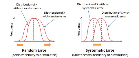
What does random and systematic error imply for measurement procedures? By increasing variability in observations, random error reduces the reliability of measurement. In contrast, by shifting the central tendency measure, systematic error reduces the validity of measurement. Validity concerns are far more serious problems in measurement than reliability concerns, because an invalid measure is probably measuring a different construct than what we intended, and hence validity problems cast serious doubt on findings derived from statistical analysis.

Note that reliability is a ratio or a fraction that captures how close the true score is relative to the observed score. Hence, reliability can be expressed as:

\[ \mbox{var}(T) / \mbox{var}(X) = \mbox{var}(T) / [ \mbox{var}(T) + \mbox{var}(E) ]\,. \]

If \(\mbox{var}(T) = \mbox{var}(X)\), then the true score has the same variability as the observed score, and the reliability is 1.0.

An integrated approach to measurement validation

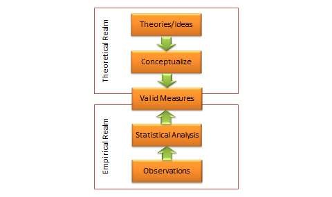
A complete and adequate assessment of validity must include both theoretical and empirical approaches. As shown in Figure 7.4, this is an elaborate multi-step process that must take into account the different types of scale reliability and validity.

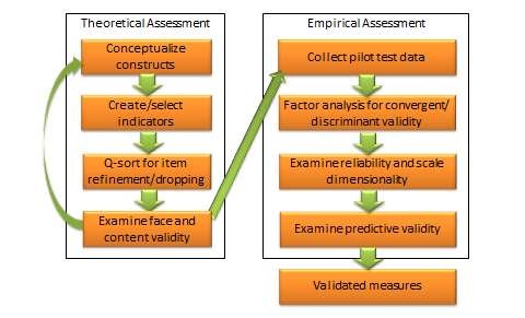
The integrated approach starts in the theoretical realm. The first step is conceptualising the constructs of interest. This includes defining each construct and identifying their constituent domains and/or dimensions. Next, we select (or create) items or indicators for each construct based on our conceptualisation of these constructs, as described in the scaling procedure in Chapter 5. A literature review may also be helpful in indicator selection. Each item is reworded in a uniform manner using simple and easy-to-understand text. Following this step, a panel of expert judges (academics experienced in research methods and/or a representative set of target respondents) can be employed to examine each indicator and conduct a Q-sort analysis. In this analysis, each judge is given a list of all constructs with their conceptual definitions and a stack of index cards listing each indicator for each of the construct measures (one indicator per index card). Judges are then asked to independently read each index card, examine the clarity, readability, and semantic meaning of that item, and sort it with the construct where it seems to make the most sense, based on the construct definitions provided. Inter-rater reliability is assessed to examine the extent to which judges agreed with their classifications. Ambiguous items that were consistently missed by many judges may be re-examined, reworded, or dropped. The best items (say 10–15) for each construct are selected for further analysis. Each of the selected items is re-examined by judges for face validity and content validity. If an adequate set of items is not achieved at this stage, new items may have to be created based on the conceptual definition of the intended construct. Two or three rounds of Q-sort may be needed to arrive at reasonable agreement between judges on a set of items that best represents the constructs of interest.

Next, the validation procedure moves to the empirical realm. A research instrument is created comprising all of the refined construct items, and is administered to a pilot test group of representative respondents from the target population. Data collected is tabulated and subjected to correlational analysis or exploratory factor analysis using a software program such as SAS or SPSS for assessment of convergent and discriminant validity. Items that do not meet the expected norms of factor loading (same-factor loadings higher than 0.60, and cross-factor loadings less than 0.30) should be dropped at this stage. The remaining scales are evaluated for reliability using a measure of internal consistency such as Cronbach alpha. Scale dimensionality may also be verified at this stage, depending on whether the targeted constructs were conceptualised as being unidimensional or multidimensional. Next, evaluate the predictive ability of each construct within a theoretically specified nomological network of construct using regression analysis or structural equation modelling. If the construct measures satisfy most or all of the requirements of reliability and validity described in this chapter, we can be assured that our operationalised measures are reasonably adequate and accurate.

The integrated approach to measurement validation discussed here is quite demanding of researcher time and effort. Nonetheless, this elaborate multi-stage process is needed to ensure that measurement scales used in our research meet the expected norms of scientific research. Because inferences drawn using flawed or compromised scales are meaningless, scale validation and measurement remains one of the most important and involved phases of empirical research.